
Shared: wetness + dye per cell
Paint a wash and let it dry
The edge dries darker, 1.3 to 2.5 times the middle, pinned by a test.
Game Tailors
Source: The science of simulating
The drawing app where the paper is real. No ads. No accounts. No personal data: only anonymous counts, which you can switch off.
Game Tailors · Schieweg 15Y-40, 2627 AN Delft (NL)
KvK 92437702 · VAT NL866044474B01
info@gametailors.com · +31 6 4227 5919
© 2026 Game Tailors
The science of simulating
Professor Oops began with a reading list: how computer-animation researchers keep simulated wind from blowing up, why a dried watercolour has a dark rim, how a forensic scientist reads the angle of a falling drop. We kept the effects people recognise and left out what costs a tablet too much. This page lists every source, what we took from it, and what we turned down and why.

The game's simulation started in October 2026 with two research notes. They went through the computer graphics and physics literature with one stated rule: believable rather than physically correct, and the cheapest technique that keeps the signatures people recognise.
A dark rim on a dried wash is a signature. So is the way a puddle runs back into the track a finger leaves, or the way a drop that lands at a slant leaves a long stain. The exact speed of a ripple on three millimetres of water is not, at least not to a child holding a tablet.
The research ended up doing three different jobs. A few methods went into the code by name. Much more shaped the idea of a system and then got built in a simpler way. And some of the best-known work was read and deliberately left out. Each source on this page carries one of four labels:
Applied directly: the code names the method and follows it
Informed the design: it shaped a decision, built or not
Found later: the code uses a classic name; the paper behind it, listed for checking
Not used yet: strong work we haven't drawn on
The third label is there for honesty. The code uses classic names such as multigrid, over-relaxation, vorticity confinement, the coffee-ring effect, Marangoni flow and Poiseuille's law without citing anyone. We list the papers behind those names so an engineer can check us, and we don't claim we followed them.
Hold a hair dryer over flour and the flour is blown off its heap and comes down further out. That wind comes from "stable fluids" Stam 1999, the one fluid method in the game applied directly. It was made for animation rather than engineering accuracy, and its selling point is that it cannot blow up, however big the time step. Each step moves the wind along itself by looking backwards to where each bit of air came from, then takes out the part of the flow that piles up.
We changed it in three places, each for a reason. Seen from above, air isn't trapped in the plane of the paper: a fan blowing down is a source, a fire drawing air up is a sink. So only part of the correction is applied, and the pressure is "screened": its reach fades over a short distance on the paper. There is no viscosity step, only a gentle overall damping. And small swirls are kept alive by vorticity confinement, a technique the code names; it goes back to Steinhoff and Underhill Steinhoff 1994 and came into graphics with Fedkiw, Stam and Jensen Fedkiw 2001.
The pressure solve has its own story. The first air used a fixed run of Gauss-Seidel sweeps, the same kind of relaxation as Stam's short recipe for games Stam 2003. We found it leaned: draughts blew about a fifth harder one way than the other, and the middle of a gust sat half a cell down and to the right of where it was blown. Gauss-Seidel updates cells in reading order, each one using neighbours already updated in the same sweep, so the answer depends on which corner you start from.
That finding was ours, not a paper's. The fix was a classic method used carefully. Multigrid Brandt 1977, Briggs 2000 smooths on the fine grid and solves what's left on coarser ones, where errors that span the page become short-range and cheap to remove. Our sweeps are Jacobi sweeps, every cell from the sweep before, and a cell's neighbours are added in pairs, so the wind mirrored left to right gets a correction mirrored to the bit.
The GPU route in our notes Harris 2004, WebGL fluid was not taken. The air runs on the CPU, in a WebAssembly kernel inside a Web Worker, and that kernel agrees with the plain JavaScript version to the bit. Jacobi was chosen there for symmetry, not for parallel hardware.
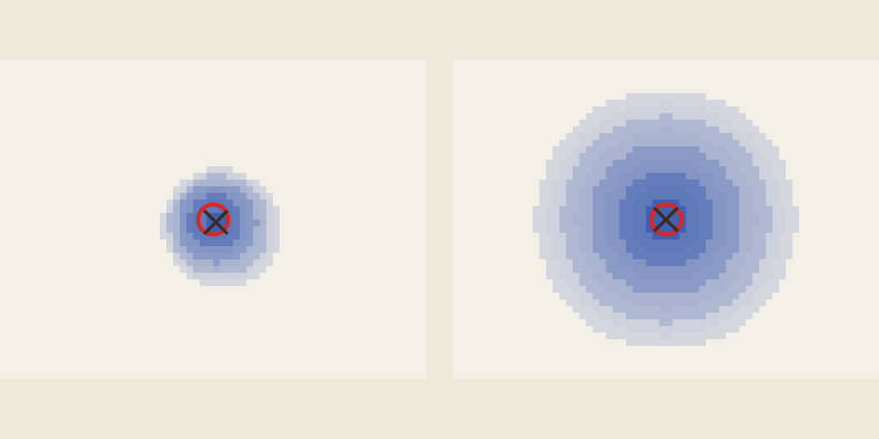
Both panes solve the same pressure for one fan on the 64 × 48 desktop air grid, from nothing, and spend the same amount of work. The multigrid pane is the game's solver step by step: coarsest grid first, then one V-cycle per level, then more V-cycles. The Gauss-Seidel pane runs the plain method on the same equation, one sweep at a time. Tap a pane to move the fan, or press Move the fan. What to look for: multigrid shows a coarse answer almost at once and its full answer after about five sweeps' worth of work, already close; Gauss-Seidel creeps outward, and its centre (the cross) sits off the fan's (the ring). Switch the screening off to see how slowly a single sweep's reach spreads across a whole page.
This part of the page could not start.
Three works we haven't drawn on would be the first checks of these choices. McAdams, Sifakis and Teran McAdams 2010 is multigrid for fluids in graphics, the nearest prior art to our solver. Bridson's textbook Bridson 2016 would question our velocities at cell centres rather than on cell faces. Chorin's 1968 paper Chorin 1968 is an ancestor of the projection step itself.
next update In the released game, standing water evens itself out at a plain rate, with no momentum. In the next update it keeps going once it's moving. Drag a finger through a puddle and the water runs back into the track at once; a thin sheen hardly moves at all.
The technique is "virtual pipes". Every cell is joined to its four neighbours by a pipe. What a pipe carries this step is what it carried last step, sped up by how much higher the water stands on one side. The idea goes back to O'Brien and Hodgins O'Brien 1995, and reached us through the hydraulic erosion work of Mei, Decaudin and Hu Mei 2007 and the small-scale shallow water of Dagenais et al. Dagenais 2018. That last one also uses half-millimetre cells and treats viscosity implicitly, as our code does, though our viscous term is derived separately, from Poiseuille's law Sutera 1993. Water as a height field at all goes back further, to Kass and Miller Kass 1990.
The rule carries real constants: gravity at its true 9.81 m/s², scaled to half-millimetre cells, and water's real viscosity of 1 mm²/s. That is also where it meets its limit. A wave on 3 mm of real water runs at 17 cm/s, ten cells in one step, faster than a step can carry and stay stable. So the push is capped. The cap always wins in practice, and waves in the game run at about 7 mm/s, some 25 times slower than real ones. The rule has the right form and real constants, and it is deliberately held back.
next update A 6 cm × 4 cm puddle about 1 mm deep, at the game's half-millimetre cells, stepped at the game's 30 passes a second. Every two and a half seconds a fingertip drags across it; drag your own finger through it too, or press Drag a finger across. What to look for: with pipes, the track fills back in almost at once. Switch to the released rule and the same track fills far more slowly. Thicken the liquid and the pipes lose their momentum. Low ridges stay put: a surface that is nearly level between neighbours is left to rest. Pipes only move water, so the total stays the same.

This part of the page could not start.
From real gravity the push per pass climbs from about 0.003 at 0.03 mm to over 10 at 1.5 mm; the game holds it at 0.2 from about 0.08 mm on.
| water depth (mm) | g·dt²·h·keep, from real g and ν | what the game uses, capped |
|---|---|---|
| 0.03 | 0.01167 | 0.01167 |
| 0.0337 | 0.01644 | 0.01644 |
| 0.0378 | 0.02316 | 0.02316 |
| 0.0424 | 0.03259 | 0.03259 |
| 0.0475 | 0.04583 | 0.04583 |
| 0.0533 | 0.06437 | 0.06437 |
| 0.0599 | 0.09027 | 0.09027 |
| 0.0672 | 0.1264 | 0.1264 |
| 0.0754 | 0.1765 | 0.1765 |
| 0.0846 | 0.246 | 0.2 |
| 0.0949 | 0.3415 | 0.2 |
| 0.1064 | 0.4723 | 0.2 |
| 0.1194 | 0.65 | 0.2 |
| 0.134 | 0.8895 | 0.2 |
| 0.1504 | 1.209 | 0.2 |
| 0.1687 | 1.63 | 0.2 |
| 0.1893 | 2.177 | 0.2 |
| 0.2124 | 2.878 | 0.2 |
| 0.2383 | 3.763 | 0.2 |
| 0.2674 | 4.86 | 0.2 |
| 0.3 | 6.196 | 0.2 |
| 0.3366 | 7.796 | 0.2 |
| 0.3777 | 9.68 | 0.2 |
| 0.4238 | 11.87 | 0.2 |
| 0.4755 | 14.37 | 0.2 |
| 0.5335 | 17.21 | 0.2 |
| 0.5986 | 20.4 | 0.2 |
| 0.6716 | 23.97 | 0.2 |
| 0.7536 | 27.94 | 0.2 |
| 0.8455 | 32.34 | 0.2 |
| 0.9487 | 37.23 | 0.2 |
| 1.0644 | 42.65 | 0.2 |
| 1.1943 | 48.66 | 0.2 |
| 1.3401 | 55.34 | 0.2 |
Source: Computed from real gravity, water's real viscosity and the game's cap, at the game's pass of 1/30 s.
A heap of ketchup stays a heap; paint spreads. In real life that's a yield stress: the paste doesn't flow until it's pushed hard enough. Lubrication theory for such thin "Bingham" sheets Liu 1989 gives a flux that depends on depth and slope, and our research note wrote it out. The code does something far simpler. Paste flows to a neighbour only where its surface stands higher by more than a per-material step, and then in proportion to the excess. Depth doesn't enter. The code calls it "Bingham-ish", and that is the honest word.
Two other papers shaped the goop the same way, as ideas. Carlson et al.'s melting and flowing Carlson 2002 was on the reading list, and we used none of its method. Our goop simply runs less the more of it has set. Sumner, O'Brien and Hodgins Sumner 1999 pushed sand, mud and snow aside as height columns and let steep columns slump; our bulldozing and slumping does the same with nothing lost, though none of their parameters are used. Heaped grains avalanche past a fixed rise per cell, the same family of threshold rule as the sandpile model of self-organised criticality Bak 1987.
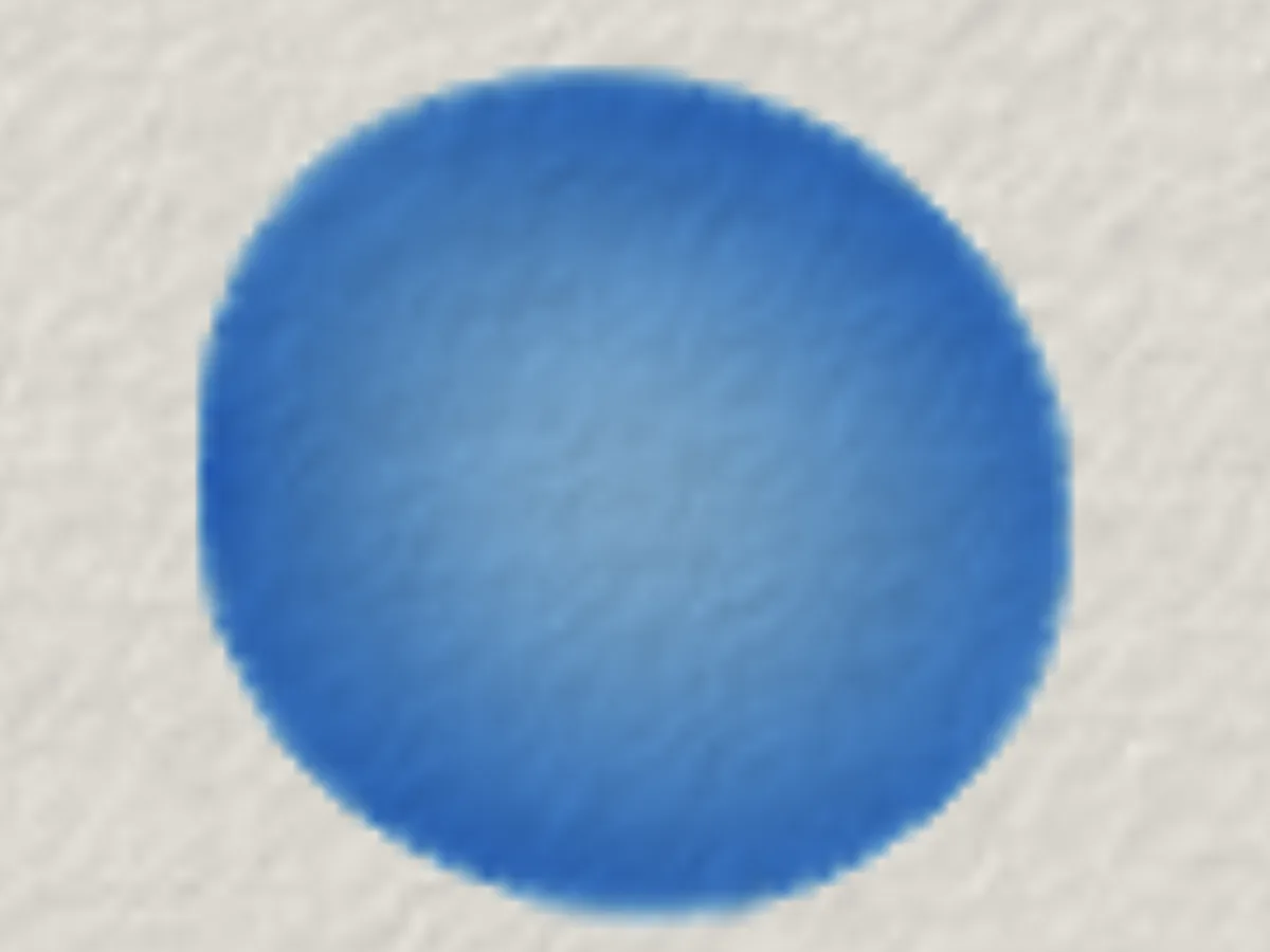
Brush a wash onto the paper, let it dry, and its edge comes out darker than its middle. Drop clean water into a drying wash and it pushes the colour out into a bloom. Those signatures come from one paper more than any other: "Computer-Generated Watercolor" by Curtis, Anderson, Seims, Fleischer and Salesin Curtis 1997. It gave us the mental model: water on the sheet, water in the fibres, pigment carried to the edges.
It did not give us its method. Curtis et al. run a small fluid simulation on the paper, with a velocity field, a mask of the wet area, an outward flow computed from a blurred mask, and glazes composited by the Kubelka-Munk optics of paint. The game has no velocity in the paper water at all. Each cell exchanges water and dye with its neighbours by their difference in wetness, gated by a fibre pattern, and every spot dries at the same rate unless it's heated. The rim appears anyway, because the thin edge empties first and water evens out toward it, bringing colour along. A test checks that the rim comes out 1.3 to 2.5 times as strong as the wash inside it.
The fibre pattern is the one thing we kept from MoXi Chu 2005, a beautiful real-time ink model built on lattice Boltzmann flow on the GPU. We parked that method as a possible special brush. What survived is its idea that noise in the fibres breaks up the wet front. The same fibre field now also sets how fast paper burns and conducts heat. The saturation-dependent spreading in our notes, which would give sharper wet fronts, was not built. Van Laerhoven and Van Reeth's real-time watery paint Van Laerhoven 2005 was in the notes too; it is GPU dynamics as well, and we took nothing specific from it.
A dried coffee drop has a dark ring for a reason explained by Deegan et al. Deegan 1997: liquid lost at a pinned edge is replaced from inside, and that flow carries the solids out. The game's grains also ride the water toward a drying edge. That's consistent in mechanism only. There's no pinned contact line, no extra evaporation at the rim, and nobody has tested the paper's power law.
Real paint scatters light as well as absorbing it. That is why light paint can cover dark. The classic model of it is Kubelka and Munk's Kubelka 1931, and our research note recommended storing its two numbers per pigment. A modern method built on it, Mixbox Sochorová 2021, mixes digital paint beautifully, but its licence is non-commercial, and that ruled it out. The open spectral.js library spectral.js was considered and not adopted.
The game does something cheaper. A colour is how much light it takes away, per red, green and blue channel. Layers add their absorbance and the light left falls exponentially with it, which is what the Beer-Lambert law describes Swinehart 1962; the code calls it optical density. Two thin washes darken together the way real ones do. What's lost is scattering: light paint can't cover dark. How colours mix has the whole model.
Water climbs into paper with its front moving as the square root of time. Lucas Lucas 1918 and Washburn Washburn 1921 worked that law out, and Richards Richards 1931 wrote the porous-flow equation in which wetter paper carries water better, the cause of a sharp wet front. Nobody has measured the game's wet front against √t yet. If it holds, it would be a real comparison with physics rather than a resemblance. Before Curtis et al., Small Small 1991 simulated watercolour on a Connection Machine; Curtis et al. call it groundbreaking, and we haven't read it.
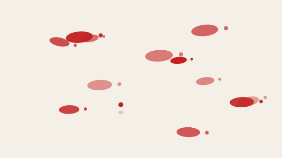
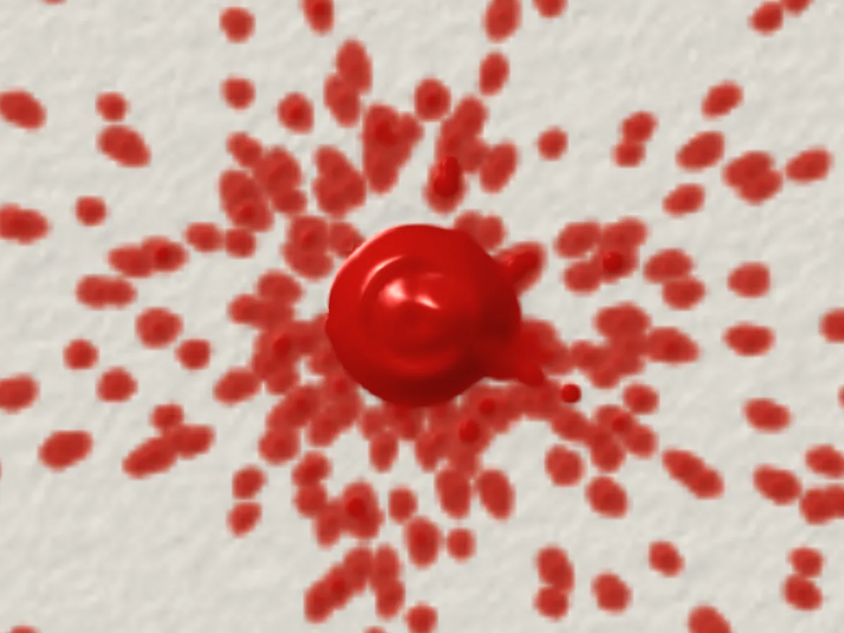
Splash paint across the page and each drop leaves a stain. A drop that comes straight down leaves a round dot; one that skims in at a low angle leaves a long oval pointing the way it was going. Crime-scene investigators use this to work out where blood came from. The rule is simple: the stain's width divided by its length is the sine of the angle the drop came in at. It's credited to Balthazard and colleagues in 1939, and we applied it directly from a fluid dynamics write-up by Neitzel and Smith Neitzel & Smith.
The game works out each drop's impact angle from its own speed across the page and its speed coming down, so a drop thrown fast and low leaves a long stain and one that falls straight down a round one. The stretch is capped, so very shallow drops don't turn into thin streaks.
The rest of the splash research in our notes we didn't build: how many fingers form round a drop hitting a plate Mehdizadeh 2004, how a crown splash's rim grows and breaks up Agbaglah 2014, and crown fingers from non-spherical drops Anirudh 2026. Splash physics of this kind weighs a drop's inertia against its surface tension, the Weber number. No Weber number exists anywhere in the code. Tails and satellite droplets come from simple rules.
Drops fly in from the left and land at the angle you set. Tap the paper to throw one at a spot, or press Throw a drop. What to look for: at 90° the stains are round; below 30° they stretch to twice their width and more; below about 14.5° they stop growing at 4 : 1, where the real rule would keep going. Turn on the outline to see the real rule's shape around the newest stain.
This part of the page could not start.
The forensic rule gives 11.5 : 1 at 5° and 2 : 1 at 30°; the game follows it down to 14.5° and stays at 4 : 1 below that.
| impact angle (degrees) | the forensic rule, 1 / sin α | the game, capped at 4 |
|---|---|---|
| 5 | 11.474 | 4 |
| 6 | 9.567 | 4 |
| 7 | 8.206 | 4 |
| 8 | 7.185 | 4 |
| 9 | 6.392 | 4 |
| 10 | 5.759 | 4 |
| 11 | 5.241 | 4 |
| 12 | 4.81 | 4 |
| 13 | 4.445 | 4 |
| 14 | 4.134 | 4 |
| 15 | 3.864 | 3.864 |
| 16 | 3.628 | 3.628 |
| 17 | 3.42 | 3.42 |
| 18 | 3.236 | 3.236 |
| 19 | 3.072 | 3.072 |
| 20 | 2.924 | 2.924 |
| 21 | 2.79 | 2.79 |
| 22 | 2.669 | 2.669 |
| 23 | 2.559 | 2.559 |
| 24 | 2.459 | 2.459 |
| 25 | 2.366 | 2.366 |
| 26 | 2.281 | 2.281 |
| 27 | 2.203 | 2.203 |
| 28 | 2.13 | 2.13 |
| 29 | 2.063 | 2.063 |
| 30 | 2 | 2 |
| 31 | 1.942 | 1.942 |
| 32 | 1.887 | 1.887 |
| 33 | 1.836 | 1.836 |
| 34 | 1.788 | 1.788 |
| 35 | 1.743 | 1.743 |
| 36 | 1.701 | 1.701 |
| 37 | 1.662 | 1.662 |
| 38 | 1.624 | 1.624 |
| 39 | 1.589 | 1.589 |
| 40 | 1.556 | 1.556 |
| 41 | 1.524 | 1.524 |
| 42 | 1.494 | 1.494 |
| 43 | 1.466 | 1.466 |
| 44 | 1.44 | 1.44 |
| 45 | 1.414 | 1.414 |
| 46 | 1.39 | 1.39 |
| 47 | 1.367 | 1.367 |
| 48 | 1.346 | 1.346 |
| 49 | 1.325 | 1.325 |
| 50 | 1.305 | 1.305 |
| 51 | 1.287 | 1.287 |
| 52 | 1.269 | 1.269 |
| 53 | 1.252 | 1.252 |
| 54 | 1.236 | 1.236 |
| 55 | 1.221 | 1.221 |
| 56 | 1.206 | 1.206 |
| 57 | 1.192 | 1.192 |
| 58 | 1.179 | 1.179 |
| 59 | 1.167 | 1.167 |
| 60 | 1.155 | 1.155 |
| 61 | 1.143 | 1.143 |
| 62 | 1.133 | 1.133 |
| 63 | 1.122 | 1.122 |
| 64 | 1.113 | 1.113 |
| 65 | 1.103 | 1.103 |
| 66 | 1.095 | 1.095 |
| 67 | 1.086 | 1.086 |
| 68 | 1.079 | 1.079 |
| 69 | 1.071 | 1.071 |
| 70 | 1.064 | 1.064 |
| 71 | 1.058 | 1.058 |
| 72 | 1.051 | 1.051 |
| 73 | 1.046 | 1.046 |
| 74 | 1.04 | 1.04 |
| 75 | 1.035 | 1.035 |
| 76 | 1.031 | 1.031 |
| 77 | 1.026 | 1.026 |
| 78 | 1.022 | 1.022 |
| 79 | 1.019 | 1.019 |
| 80 | 1.015 | 1.015 |
| 81 | 1.012 | 1.012 |
| 82 | 1.01 | 1.01 |
| 83 | 1.008 | 1.008 |
| 84 | 1.006 | 1.006 |
| 85 | 1.004 | 1.004 |
| 86 | 1.002 | 1.002 |
| 87 | 1.001 | 1.001 |
| 88 | 1.001 | 1.001 |
| 89 | 1 | 1 |
| 90 | 1 | 1 |
Source: The rule as given by Neitzel & Smith, and the game's capped version of it.
Leave food out on the page, skip ahead three days, and fuzzy mould colonies have spread over it. Real mould grows as branching threads. The textbook way to grow branching shapes in a computer is diffusion-limited aggregation Witten 1981: particles wander at random until they touch the cluster and stick. It makes lovely, lifelike fronds.
We turned it down for two reasons. Literal random walkers are slow, and a time skip would mean simulating every hour of the three days. Instead each colony's radius is a formula of its age. "Come back three days later" is one sum per colony, not three days of work, which is exactly what our research note asked for.
Other pattern makers were noted and not built either: Gray-Scott reaction-diffusion as Karl Sims's tutorial presents it Sims, and the slime-mould transport networks of Jones Jones 2010. Turing's 1952 paper on patterns from reaction and diffusion Turing 1952 is the classic behind the first. (A comment in the fire code says "reaction-diffusion", but it means heat and fuel; the fire is a travelling front, not a Turing pattern.)
The game's own rule Two colonies on the same clock, four sim-hours a second. The random walkers grow by diffusion-limited aggregation: walkers wander until they touch the colony and stick. The other pane is the game's formula for a typical colony. Each frame the walkers get a fixed budget of steps, as a device would. What to look for: press "Come back in 3 days". The formula jumps there at once; the walkers have to catch up step by step, and the step counter shows the bill. Lower the budget to play a slower tablet.
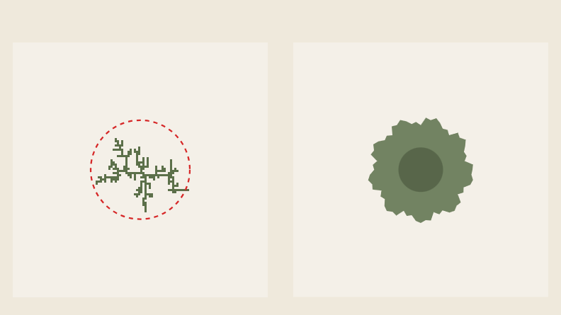
This part of the page could not start.
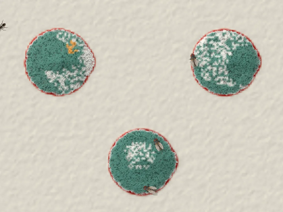
Hold a match to paper and a ragged front eats outward, with a blackened edge. We read up on burning paper in graphics: three papers by Melek and Keyser, one of them on bending burning matches and crumpling burning paper Melek 2005, Melek 2006, Melek 2007, and Larboulette, Quesada and Dumas, who burn paper fibre by fibre Larboulette 2013. Our research note turned down that paper's curling sheet of masses and springs as overkill, in writing. A clean example of a source consulted and declined.
The game's fire is heat spreading through the paper, with fuel that burns away. Paper catches at a fixed threshold, about 230 °C; the randomness sits instead in the fuel and in burn rates tied to the fibre field. There's no oxygen field: carbon dioxide and anything lying on top stand in for "no air". Water holds a cell at boiling until it has dried. No line sets the speed of the front, yet it comes out at about 1.1 mm a second, the same order as one published measurement for paper. It wasn't calibrated to it.
Strong fire work we haven't drawn on: Rothermel's classic spread model for wildland fires Rothermel 1972, at the wrong scale for paper but useful as a concept; flames in graphics Nguyen 2002; and two physics papers on slowly burning paper fronts Maunuksela 1997, Zik 1998.
Draw a copper wire from a battery to a bulb and the bulb lights. The game solves for the voltage in every cell of the sheet, with each cell's real conductance, until the current balances. Engineers know the method as successive over-relaxation Young 1954. The very problem of current spreading through a flat plate was the subject of a paper Kirchhoff wrote as a student in 1845 Kirchhoff 1845. We didn't follow either paper; these are the classic names for what the code does. The answer matches Ohm's law to three figures: 0.273 A through copper and a bulb.
Drop washing-up liquid onto milk with colour on it and the colours burst away from it, then stop. That's Marangoni flow Scriven 1960: soap lowers the surface tension and the surface pulls away toward where it's higher. In the game the milk's fat takes up the soap, so the burst stops by itself. A real soluble surfactant drives a flow of finite size Roché 2014; ours also clears a finite patch and eases out, consistent in kind. Nobody has compared it with that paper's scaling laws, which makes it a good candidate for a real test.
Some of the most useful sources weren't papers at all. Falling-sand games have spent years on the question of how many materials can meet without anyone writing every pair.
Sandspiel Bittker 2019 packs each cell into 32 bits: a species, two registers and a clock. The Powder Toy Powder Toy keeps each element as a flat record of properties; its water next to salt has a 1 in 50 chance of becoming salt water. We went another way: Professor Oops isn't a cellular automaton of discrete species. Each cell carries many continuous layers, such as water, heat, dye and dissolved substances, because a wash of colour or a slowly drying puddle needs amounts, not types.
Noita Purho 2019 showed how a big sand world stays fast: only redraw and recompute the rectangles that changed. We built the same idea our own way, with small square tiles where calm ones are worked only every few passes. Nothing in the code says it came from Noita, so we don't claim it did.
The biggest idea came from a talk on The Legend of Zelda: Breath of the Wild Dohta 2017, as our notes summarised it: send interactions through shared elements, so the number of rules grows as elements times materials instead of materials times materials. The game's dissolved elements and its data-driven reaction table are built that way. That is how vinegar fizzes on baking soda and lemon turns red cabbage pink: acid, baking soda's base and the cabbage's colour are shared elements, so any material that carries them joins in. Built for surprises tells that story.
Dark blue: busy, every pass. Pale blue: settling, every few passes. Paper: still, asleep until woken. Illustration of the game's tile clock: a puddle spreading in one corner and a candle burning in another, on a page cut into tiles.
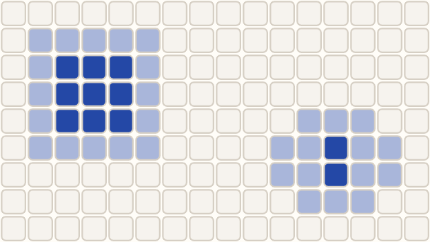
This part of the page could not start.
Each source on this page ends up in a chapter of its own. These are the threads, with the test that holds each one.
Shared: wetness + dye per cell
The edge dries darker, 1.3 to 2.5 times the middle, pinned by a test.
Shared: the wind field u, v
The flour is blown off its heap and comes down further out, and a test holds the pressure solve mirror-exact to the bit.
Shared: water depth + pipe flows
next update The water runs back into the track, measured by a test.
Shared: conductance per cell
The current settles by over-relaxation and matches Ohm's law to three figures, checked by a test.
Shared: water + heat + fibre
Soaked paper won't light: its water holds it at boiling until it has dried, pinned by a test.
Shared: surface tension field
Colours burst away and stop as the fat binds the soap, pinned by a test.
Grouped by system. Each says how it was used. Most were checked by record and abstract; the four read in full are marked. A source listed here that we haven't used is listed as a gap, never as an influence.
Applied directly. What we did: the wind's semi-Lagrangian advection and pressure projection, named in the code. Departures: no viscous diffusion, only part of a screened correction.
Informed the design · read in full. What we did: recommended in the notes for smoke. The first air's Gauss-Seidel sweeps resembled its recipe; they have since been replaced.
What we did: GPU route not taken; the air runs on the CPU and in WebAssembly. Our Jacobi sweeps are there for mirror symmetry.
What we did: a reference implementation in the notes; not used.
Found later · read in full. What we did: the code names vorticity confinement and uses a force of the same shape, gated on speed. The repo never cites this paper.
What we did: the origin of the technique above.
What we did: a foundational multigrid paper; our solver names multigrid and cites nothing.
What we did: the standard introduction to V-cycles and full multigrid; good reading for anyone checking our solver.
Not used yet. Multigrid for fluids in graphics: the nearest prior art to our solver.
Not used yet. The standard text; it would be the first check of the air's choices, including velocity at cell centres rather than on faces.
Not used yet. An ancestor of the projection step.
Found later · read in full. What we did: the origin of virtual pipes, per later sources. Our rule has its form, with four neighbours instead of eight and a viscous hold next update.
What we did: the notes' pointer to virtual pipes, for thick layers. The pipes went in by name next update; nothing shows this paper's formulas were used.
What we did: same 0.5 mm cell and implicit viscosity next update, though our term is derived from Poiseuille. Its extended pipes and multi-layer heightmaps were not built.
What we did: the ancestor of water as a height field.
What we did: the code names Poiseuille's 3ν/h² and computes it from water's real ν next update; this review is a citable history of the law.
What we did: the idea of a threshold, yes; the flux formula, no.
What we did: not its method. Our goop simply moves less as it sets.
What we did: pushing material aside as height columns and slumping steep ones, with nothing lost. None of its parameters are used.
Not used yet. The sandpile model: the same family of threshold rule as our grain slump.
Informed the design · read in full. What we did: the most important single influence on the paper model, for its behaviours. None of its method: no velocity layer, mask, blur or glazing.
What we did: in the notes; no GPU dynamics and no Kubelka-Munk built.
What we did: kept the fibre noise that gates the flow; lattice Boltzmann parked as a possible special brush.
What we did: the code says "coffee-ring effect". Consistent in mechanism only: no pinned line, no edge evaporation peak, no power-law test.
Not used yet. Watercolour on a Connection Machine, which Curtis et al. call groundbreaking.
Not used yet. The √t law of capillary rise.
Not used yet. Front distance as √t. The most useful gap: nobody has measured the game's front against it.
Not used yet. Diffusivity that depends on saturation: the formal version of the D ∝ water² we didn't build, and the cause of sharp wet fronts.
Informed the design, not built. What we did: the notes recommended K and S per pigment; the code has neither, and no scattering term.
Informed the design, not built. What we did: Mixbox; ruled out by its non-commercial licence.
Informed the design, not built. What we did: considered; not in the app. (Its README describes seven primary curves sampled at 38 points from 380 to 750 nm, with single-constant Kubelka-Munk.)
What we did: the game's colour is what the law describes: absorbance adds, light is exp(−absorbance), per channel. The code calls it optical density.
What we did: the code names the flow and cites nothing.
What we did: our clearing is also finite and eases out, consistent in kind. Not compared with its scaling laws: a good candidate for a real test.
Applied directly. What we did: sin α = W/L for every drop stain, with a cap on the stretch.
What we did: in the notes; no Weber number in the code.
What we did: in the notes; not built as a rule.
What we did: in the notes; not built as a rule.
Informed the design, rejected. What we did: walkers judged too slow; mould's radius is a formula of age instead.
Informed the design, not built. What we did: Gray-Scott noted as an idea; not in the sim.
Informed the design, not built. What we did: a bonus idea in the notes; not built.
Not used yet. The classic paper on patterns from reaction and diffusion.
What we did: consulted for burning paper; no deformation from burning built.
What we did: as above.
What we did: as above.
Informed the design, rejected. What we did: its mass-spring curling turned down in writing as overkill.
Not used yet. The classic wildland spread model: moisture, wind, slope. The wrong fuel scale for paper; useful as a concept.
Not used yet. Fire in graphics: flames rather than fronts on paper.
Not used yet. A lead on burning fronts in paper; not read.
Not used yet. A lead on burning fronts; not read.
What we did: a historical aside. It is about what the game does, current spreading across a flat sheet; the repo names only Kirchhoff's laws.
What we did: the circuit uses over-relaxation, forward then back; no citation in the repo.
What we did: read for cell layout; we chose many continuous fields per cell over discrete species.
What we did: materials as flat property records.
What we did: the idea of working only what changed, as described in an 80.lv interview with Purho. Our tiles were built our own way; nothing says they came from Noita.
What we did: elements × materials, through secondary notes: the dissolved elements and the data-driven reaction table.